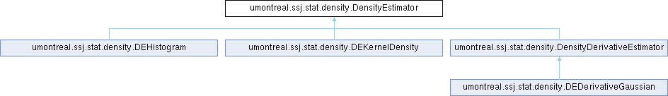
This abstract class represents a univariate density estimator (DE). More...

Inheritance diagram for DensityEstimator:

Public Member Functions
abstract void	setData (double[] data)
	Sets the observations for the density estimator do data. More...

double []	getData ()
	Gives the observations for this density estimator, if any. More...

abstract double	evalDensity (double x)
	Evaluates the density estimator at x. More...

double []	evalDensity (double[] evalPoints)
	Evaluates the density estimator at the points in evalPoints. More...

double []	evalDensity (double[] evalPoints, double[] data)
	Sets the observations for the density estimator to data and evaluates the density at each point in evalPoints. More...

double [][]	evalDensity (double[] evalPoints, double[][] data)
	This method is particularly designed to evaluate the density estimator in such a way that the result can be easily used to estimate the empirical IV and other convergence-related quantities. More...

abstract String	toString ()
	Gives a short description of the estimator. More...

Static Public Member Functions
static void	evalDensity (ArrayList< DensityEstimator > listDE, double[] evalPoints, double[][] data, ArrayList< double[][]> listDensity)
	This function is particularly designed for experiments with many different types of density estimators, as it evaluates all of these estimators at the points in evalPoints. More...

static double []	computeVariance (double[][] density)
	This method computes the empirical variance based on the values given in data. More...

static double	computeIV (double[][] density, double a, double b, double[] variance)
	This method estimates the empirical IV over the interval \([a,b]\). More...

static void	computeIV (ArrayList< double[][]> listDensity, double a, double b, ArrayList< Double > listIV)
	This method estimates the empirical IV over the interval \([a,b]\) for a collection of different estimators. More...

static double []	computeMISE (ContinuousDistribution dist, double[] evalPoints, double[][] density, double a, double b, double[] variance, double[] sqBias, double[] mse)
	In situations where the true density is known this method can estimate the empirical MISE over the interval \([a,b]\). More...

static void	computeMISE (ContinuousDistribution dist, double[] evalPoints, ArrayList< double[][]> listDensity, double a, double b, ArrayList< double[]> listMISE)
	This method estimates the empirical MISE over the interval \([a,b]\) for a collection of different estimators. More...

static String	plotDensity (double[] evalPoints, double[] density, String plotTitle, String[] axisTitles)
	Gives a plot of the estimated density. More...

static double	roughnessFunctional (double[] density, double a, double b)
	Estimates the roughness functional. More...

Protected Attributes
double []	data
	The data associated with this DensityEstimator object, if any.

Detailed Description

This abstract class represents a univariate density estimator (DE).

Both static and non-static methods are offered.
In a majority of cases, on simply wishes to estimate the density at a finite set of evaluation points, from a given set of data, and perhaps plot the estimated density. To do that, there is no need to create an object. One can simply use a static evalDensity method followed by plotDensity. Note that calling the evalDensity method only once for a vector of evaluation points is typically much faster than calling it separately for each evaluation point.

In case one plans to evaluate the same density several times with the same data, then it may be worthwhile to construct a DensityEstimator object and build the density estimate from the given data. After that, one can evaluate the density at any given point, often much faster than by calling the static method. In the case of a histogram or average shifted histogram, for example, constructing the density estimator takes time, but once it is constructed, evaluating it is relatively fast. For a KDE with fixed bandwidth, the difference (or gain) may be small.

In a non-abstract subclass, it suffices (in principle) to implement the abstract method evalDensity(double), which evaluates the density at a single point \(x\) given the data points. However, other methods will typically be overridden to make them more efficient. For example, evaluating the DE over a set of evaluation points \(\{x_0, x_1, \dots, x_{k-1}\} \) can often be performed more efficiently than by calling evalDensity(x) repeatedly in a loop.

More precisely, the single point evaluation evalDensity(double) is abstract, since it will definitely differ between subclasses. For the evaluation on a set of points one can use evalDensity(double[]). Even though a default implementation is provided, very often specific estimators will have more efficient evaluation algorithms. So, overriding this method can be beneficial in many cases. Furthermore, this class includes a method to plot the estimated density.

Another important abstract method is setData, which allows to change the observations that define the density estimator. This can be especially useful when one intends to evaluate the same type of density estimator for different sets of observations.

This class also provides more elaborate methods that deal with the convergence behavior of the DEs in terms of their IV, ISB, and MISE. As these only require evaluations of the density estimator, they are implemented as static methods.

One such method estimates the empirical IV by evaluating the empirical variance at set (or grid) of evaluation points and averaging.
See the methods computeIV, which can do that for one DE or for a list of several DEs. The MISE can also be estimated in situations where either the ISB is known to be zero or the true density is known. The methods computeMISE do that for the second case.

Member Function Documentation

◆ computeIV() [1/2]

static double computeIV	(	double	density[][],
		double	a,
		double	b,
		double []	variance
	)

static

This method estimates the empirical IV over the interval \([a,b]\).

Based on the density estimates of \(m\) independent replications of the density estimator evaluated at \(k\) evaluation points, which are provided by density, it computes the empirical variance at each evaluation point and stores it in variance.

To estimate the empirical IV, we sum up the variance at the evaluation points \(x_1,x_2,\dots,x_k\) and multiply by \((b-a)/k\), i.e.

\[ \int_a^b \hat{f}(x)\mathrm{d}x \approx \frac{b-a}{k} \sum_{j = 1}^k\hat{f}(x_j), \]

where \(\hat{f}\) denotes the density estimator. In other words, we approximate the empirical IV by an equally weighted quadrature rule using the aforementioned evaluation points as integration nodes.

Note that this is only an approximation of the true empirical IV and that the approximation quality significantly depends on the choice of evaluation points.

The data for the variance are given in the two-dimensional \(m\times k\) array density, which is also described in computeVariance(double[][]) and can be obtained by evalDensity(double[], double[][]) . The boundaries of the interval are given by a and b. Note that the array variance needs to be of length \(k\).

Parameters

density	the \(m\times k\) array that contains the data of evaluating \(m\) replicates of the density estimator at \(k\) evaluation points
a	the left boundary of the interval.
b	the right boundary of the interval.
variance	the array of length \(k\) in which the variance at each evaluation point is stored.

Returns: the estimated empirical IV over \([a,b]\).

◆ computeIV() [2/2]

static void computeIV	(	ArrayList< double[][]>	listDensity,
		double	a,
		double	b,
		ArrayList< Double >	listIV
	)

static

This method estimates the empirical IV over the interval \([a,b]\) for a collection of different estimators.

In densityList the user passes a list of \(m\times k\) arrays which contain the density estimates of \(m\) independent replications of each density estimator evaluated at \(k\) evaluation points. Such a list can be obtained via evalDensity(ArrayList, double[], double[][], ArrayList) , for instance.

The method then calls computeIV(double[][], double, double, double[]) for each element of densityList and adds the thereby obtained estimated empirical IV to the list that is being returned.

Parameters

listDensity	list containing \(m\times k\) arrays that contain the data of evaluating \(m\) replicates of each density estimator at \(k\) evaluation points evalPoints.
a	the left boundary of the interval.
b	the right boundary of the interval.
listIV	the list to which the estimated empirical IV of each density estimator will be added.

Remarks: Florian: I kept the return type as "void" instead of "ArrayList<double[][]>" and pass the corresponding list listDensity to allow for more flexibility when working with it.

◆ computeMISE() [1/2]

static double [] computeMISE	(	ContinuousDistribution	dist,
		double []	evalPoints,
		double	density[][],
		double	a,
		double	b,
		double []	variance,
		double []	sqBias,
		double []	mse
	)

static

In situations where the true density is known this method can estimate the empirical MISE over the interval \([a,b]\).

This can be particularly interesting and useful for testing density estimators. Since it is necessary to compute either the ISB or the IV to get the MISE and as there is not much computational overhead to estimate the other, an array containing the estimated empirical IV, the ISB, and MISE in exactly this order is returned. Based on the density estimates of \(m\) independent replications of the density estimator evaluated at \(k\) evaluation points evalPoints, which are provided by density, it computes the empirical variance, the square-bias, and the mean square error (MSE) at each evaluation point and stores the result in variance, sqBias, and mse, respectively. It is important that the evaluation points in evalPoints are the same as the ones used to construct density.

To estimate the empirical IV and MISE we sum up the variance and the MSE at the \(k\) evaluation points and multiply by \((b-a)/k\), i.e. we approximate the empirical IV by an equally weighted quadrature rule with evalPoints as integration nodes. The ISB is then computed as the difference of the MISE and the IV. Note that this is only an approximation of the true empirical values and that the approximation quality significantly depends on the choice of evalPoints.

The data for the variance and mse are given in the two-dimensional \(m\times k\) array density, which is also described in computeVariance(double[][]) and can be obtained by evalDensity(double[], double[][], double, double), and the true density is passed via a umontreal.ssj.probdist.ContinuousDistribution. The evaluation points are contained in evalPoints and the boundaries of the interval over which we estimate are given by a and b. Note that the arrays variance, sqBias, and mse all need to be of length \(k\).

Parameters

dist	the true density.
evalPoints	the \(k\) evaluation points.
density	the \(m\times k\) array that contains the data of evaluating \(m\) replicates of the density estimator at \(k\) evaluation points evalPoints.
a	the left boundary of the interval.
b	the right boundary of the interval.
variance	the array of length \(k\) in which the variance at each evaluation point is stored.
sqBias	the array of length \(k\) in which the square-bias at each evaluation point is stored.
mse	the array of length \(k\) in which the MSE at each evaluation point is stored.

Returns: an array containing the estimated empirical IV, ISB, and MISE in exactly this order.

◆ computeMISE() [2/2]

static void computeMISE	(	ContinuousDistribution	dist,
		double []	evalPoints,
		ArrayList< double[][]>	listDensity,
		double	a,
		double	b,
		ArrayList< double[]>	listMISE
	)

static

This method estimates the empirical MISE over the interval \([a,b]\) for a collection of different estimators.

This can be done when the true density is actually known and is particularly interesting and/or useful for testing density estimators.

In densityList the user passes a list of \(m\times k\) arrays which contain the density estimates of \(m\) independent replications of each density estimator evaluated at \(k\) evaluation points. Such a list can be obtained by calling evalDensity(ArrayList, double[], double[][], ArrayList), for instance.

The method then calls computeMISE(ContinuousDistribution, double[], double[][], double, double, double[], double[], double[]) for each element of listDensity. This results in an array containing the estimated empirical IV, ISB, and MISE in exactly this order, which is then added to the list listMISE.

Parameters

dist	the true density.
evalPoints	the \(k\) evaluation points.
listDensity	list of \(m\times k\) arrays that contain the data of evaluating \(m\) replicates of each density estimator at \(k\) evaluation points evalPoints.
a	the left boundary of the interval.
b	the right boundary of the interval.
listMISE	a list to which the arrays containing the estimated empirical IV, ISB, and MISE of each density estimator are added.

Remarks: Florian: I kept the return type as "void" instead of "ArrayList<double[][]>" and pass the corresponding list listDensity to allow for more flexibility when working with it.

◆ computeVariance()

static double [] computeVariance ( double density[][] )

static

This method computes the empirical variance based on the values given in data.

More precisely, density is a \(m\times k\) matrix, whose entries correspond to \(m\) independent realizations of the density estimator, each evaluated at \(k\) evaluation points. Such a matrix can, for instance, be obtained by evalDensity(double[], double[][]).

The empirical variance is computed at each of those \(k \) evaluation points and returned in an array of size \(k\).

Parameters

density the estimated density of \(m\) independent realizations of the estimator, each evaluated at \(k\) evaluation points.

Returns: the empirical variance at those \(k\) evaluation points.

◆ evalDensity() [1/5]

abstract double evalDensity ( double x )

abstract

Evaluates the density estimator at x.

Parameters

x	the evaluation point.

Returns: the density estimator evaluated at \(x\).

◆ evalDensity() [2/5]

double [] evalDensity ( double [] evalPoints )

Evaluates the density estimator at the points in evalPoints.

By default, this method calls evalDensity(double) for each entry of evalPoints. Many density estimators can handle evaluation at a set of points more efficiently than that. If so, it is suggested to override this method in the implementation of the corresponding estimator.

Returns: the density estimator evaluated at the points evalPoints.

◆ evalDensity() [3/5]

double [] evalDensity	(	double []	evalPoints,
		double []	data
	)

Sets the observations for the density estimator to data and evaluates the density at each point in evalPoints.

Parameters

evalPoints	the evaluation points.
data	the observations.

Returns: the density estimator defined by data evaluated at each point in evalPoints.

◆ evalDensity() [4/5]

double [][] evalDensity	(	double []	evalPoints,
		double	data[][]
	)

This method is particularly designed to evaluate the density estimator in such a way that the result can be easily used to estimate the empirical IV and other convergence-related quantities.

Assume that we have \(m\) independent realizations of the underlying model. For each such realization this method constructs a density and evaluates it at the points from evalPoints. The independent realizations are passed via the 2-dimensional \(m\times n\) array data, where \(n\) denotes the number of observations per realization. Hence, its first index identifies the independent realization while its second index identifies a specific observation of this realization.

The result is returned as a \(m\times k\) matrix, where \(k \) is the number of evaluation points, i.e., the length of evalPoints. The first index, again, identifies the independent realization whereas the second index corresponds to the point of evalPoints at which the density estimator was evaluated.

Parameters

evalPoints	the evaluation points.
data	the two-dimensional array carrying the observations of \(m\) independent realizations of the underlying model.

Returns: the density estimator for each realization evaluated at evalPoints.

◆ evalDensity() [5/5]

static void evalDensity	(	ArrayList< DensityEstimator >	listDE,
		double []	evalPoints,
		double	data[][],
		ArrayList< double[][]>	listDensity
	)

static

This function is particularly designed for experiments with many different types of density estimators, as it evaluates all of these estimators at the points in evalPoints.

To this end, the user passes a list of density estimators in listDE as well as \(m\) independent realizations of the underlying model consisting of \(n\) observations each in the \(m\times n\) array data.

This method then calls evalDensity(double[], double[][]) for each density estimator in listDE, thus evaluating the respective density estimator at the \(k\) points in evalPoints and adds the resulting \(m\times k\) array to listDensity.

Parameters

listDE	the list of density estimators.
evalPoints	the evaluation points.
data	the two-dimensional array carrying the observations of \(m\) independent realizations of the underlying model.
listDensity	a list to which the evaluations at evalPoints of each density estimator in listDE are added.

Remarks: Florian: I kept the return type as "void" instead of "ArrayList<double[][]>" and pass the corresponding list listDensity to allow for more flexibility when working with it.

◆ getData()

double [] getData ( )

Gives the observations for this density estimator, if any.

Returns: the observations for this density estimator.

◆ plotDensity()

static String plotDensity	(	double []	evalPoints,
		double []	density,
		String	plotTitle,
		String []	axisTitles
	)

static

Gives a plot of the estimated density.

The \(x\)-values are passed in evalPoints and the \(y\)-values in density. The user may also set the title of the plot via plotTitle as well as the names of the axes via axisTitles. The latter contains the name of the \(x\) axis as first element and the name of the \(y\) axis as second.

The plot itself is returned as a string, which forms a stand-alone LaTex file (including necessary headers) implementing a tikZ picture.

This function merely tailors and simplifies the methods provided by umontreal.ssj.stat.PgfDataTable for the purpose of plotting a univariate function. If the user seeks to produce more sophisticated plots, please refer to the aforementioned class.

Parameters

evalPoints	the \(x\)-values.
density	the \(y\)-values.
plotTitle	the title of the plot.
axisTitles

Returns

◆ roughnessFunctional()

static double roughnessFunctional	(	double []	density,
		double	a,
		double	b
	)

static

Estimates the roughness functional.

\[ R(g) = \int_a^b g^2(x)\mathrm{d}x\]

of a function \(g\) over the interval \([a,b]\). This is done via a quadrature rule using predetermined values of \(g\) passed by the user via density as integration nodes.

Parameters

density	the function evaluations.
a	the left boundary of the interval
b	the right boundary of the interval

Returns

◆ setData()

abstract void setData ( double [] data )

abstract

Sets the observations for the density estimator do data.

Note that, in some cases, this requires to completely reconstruct the density estimator.

Parameters

data	the desired observations.

◆ toString()

abstract String toString ( )

abstract

Gives a short description of the estimator.

Returns: a short description.

The documentation for this class was generated from the following file:

DensityEstimator.java

Public Member Functions

Static Public Member Functions

Protected Attributes

Detailed Description

Member Function Documentation

◆ computeIV() [1/2]

◆ computeIV() [2/2]

◆ computeMISE() [1/2]

◆ computeMISE() [2/2]

◆ computeVariance()

◆ evalDensity() [1/5]

◆ evalDensity() [2/5]

◆ evalDensity() [3/5]

◆ evalDensity() [4/5]

◆ evalDensity() [5/5]

◆ getData()

◆ plotDensity()

◆ roughnessFunctional()

◆ setData()

◆ toString()